Fundamentals of Neural Recording
1. Non-invasive vs. Invasive Recording Methods
| Feature | Non-invasive Methods | Invasive Methods |
|---|---|---|
| Examples | fMRI, EEG, MEG | Intracellular / Extracellular Recording |
| Sensor Location | Outside the skull (Scalp) | Inside the skull (Intracranial) |
| Primary Subjects | Can be humans | Usually animals (Rodents, Primates) |
| Analogy | The Concert Hall The singer hears the general atmosphere (roar of the crowd) but cannot distinguish individuals. | The Interview The interviewer holds a microphone to a specific person to hear exactly what they say. |
| Resolution | Aggregated Signal Reads a large pool of neurons; cannot isolate single units. | Single Unit Can isolate and record from individual neurons. |
2. Types of Invasive Recording: Intracellular vs. Extracellular
Invasive recordings are further categorized by where the electrode is placed relative to the cell membrane. When an action potential occurs and propagates along the axon, the sudden influx of sodium ions creates a positive charge inside the cell, leaving the external environment relatively negative. Consequently, the action potential appears as a positive deflection when measured intracellularly, but as a negative deflection when recorded extracellularly.
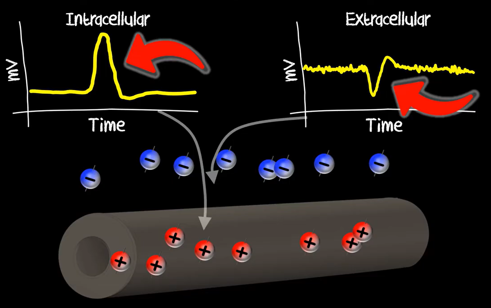
| Feature | Intracellular Recording | Extracellular Recording |
|---|---|---|
| Electrode Placement | Inside the cell membrane | Outside (adjacent to) the cell membrane |
| Signal Source | Single Neuron (Membrane Potential) | Aggregate of nearby neurons + LFP |
| Waveform Polarity | Positive (Upward deflection) | Negative (Downward/Flipped deflection) |
| Signal Strength | Strong (mV range), High Fidelity | Weak ((\mu)V range), Noisy |
| Key Challenge | Stability: Difficult to maintain in moving animals (fragile) | Separation: Requires Spike Sorting to distinguish individual neurons |
| Key Advantage | Measures exact membrane potential (sub-threshold) | Robust: Suitable for long-term recording in awake, behaving animals |
| Common Techniques | Patch Clamp, Sharp Microelectrode | Tetrodes, Silicon Probes, Microwire Arrays |
| Data Types | (V_m) (Membrane Voltage) | LFP, MUA (Multi-Unit), SUA (Single-Unit) |
Note: When we say “single unit recording,” we generally refer to invasive, extracellular recording. It does not mean that we record from a single neuron. Rather, it means we record multiple neurons but we can isolate each neuron’s activity from the aggregated signal.
3. Preprocessing for Extracellular Recording
Because the signal is measured from outside the cell, it has four distinct characteristics: “Flipped, Noisy, Weak, Aggregated.”
- Flipped: Since the electrode is outside, the action potential appears as a negative deflection (convex down). You must look for “dips” rather than peaks.
- Noisy: Contains significant background electrical noise.
- Weak: The signal amplitude is very low.
- $\rightarrow$ Requires Filtering.
- Aggregated: A single electrode picks up spikes from multiple neighboring neurons.
- $\rightarrow$ Requires Spike Sorting.
A common preprocessing pipeline for extracellular recording includes these three key steps:
- Filtering: Separates the raw signal into meaningful frequency bands:
- LFP (Local Field Potential): < 300 Hz (captures slower synaptic potentials).
- Spiking Activity (MUA/SUA): 300 – 3,000 Hz (isolates fast action potentials).
- Spike Detection: Identifies potential waveforms by setting a threshold (typically 3–4x the standard deviation of the noise) to find signals that stand out from the background noise.
- Spike Sorting: Clusters the detected waveforms based on their shape and features (like PCA components) to assign each spike to a specific, unique neuron.
4. Spike Sorting
The process of separating the activity of individual neurons from the aggregated signal.
Step 1: Spike Detection
- Identify waveforms that are significantly larger than the background noise.
- Threshold: Usually set to 3x or 4x the Standard Deviation (SD) of the noise.
Step 2: Sorting / Clustering
- Group the detected waveforms based on their shape to assign them to specific neurons.
- Technique: Dimensionality reduction (e.g., PCA) followed by clustering.
- Features: Amplitude, width, and waveform shape are key discriminators.
5. Visualization: Raster Plot
The standard method for visualizing spike timing data.
- Structure:
- X-axis: Time.
- Y-axis: Trial number.
- Dots: Occurrence of a spike.
- Interpretation:
- Annotations: Stimulus onset or behavioral events are usually marked at the top.
- Vertical Patterns: Reveal consistency across trials (Do spikes align at the same time relative to the stimulus?).
- Horizontal Patterns: Reveal temporal patterns (Is the neuron bursting? Is it tonic?).
Reference
-
“Single-Unit Recording Explained! Neuroscience Methods 101.” YouTube, uploaded by Psyched!, 24 July 2022, www.youtube.com/watch?v=LyBPd53cSPI.
Enjoy Reading This Article?
Here are some more articles you might like to read next: