Fundamentals of Diffusion Map Embedding

Principles and practice of nonlinear dimensionality reduction popularly used in neuroscience.

The Diffusion Map Workflow

Input: Data in ambient dimension (of any type that a kernel can be defined).

1. Pairwise Distance Matrix: an $n \times n$ matrix, $(i,j)$-th entry is the distance between $X_i$ and $X_j$.
2. Affinity Matrix: Perform an entry-wise evaluation using a kernel function (typically Gaussian) to convert distances into affinities. Affinity captures the local geometric structure of the data and ignores the global structure.
3. Transition Matrix ($P$): Row-normalize the affinity matrix to create the stochastic transition matrix $P$, often referred to as the diffusion operator. This matrix defines the probability of a “random walk” jumping from one data point to another in a single step.
4. Spectral Decomposition: Perform an eigendecomposition on $P$. We focus on the non-trivial eigenvectors ${\psi_1, \psi_2, \dots, \psi_k}$ (excluding the constant $\psi_0$). The $i$-th entry of each eigenvector, scaled by its corresponding eigenvalue $\lambda^t$, serves as the new coordinate for the $i$-th data point.

Output: $k$-dimensional Euclidean vectors representing the data on the underlying manifold.

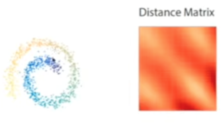
Distance Matrix

For Euclidean data, the entries of the distance matrix are defined as: \(D(x_i, x_j) = \sqrt{\|x_i - x_j\|^2}\) However, the data can be of any type, provided a suitable kernel can be defined to measure similarity. In the distance matrix below, we observe a banded pattern extending across the entire matrix. indicating a global structure.

Distance matrix

Affinity Matrix

The pairwise distances are then passed through a nonlinear kernel function to calculate affinities. The nonlinearity effectively preserves local geometric information by giving higher weight to nearby points. For example, using a Gaussian kernel: \(A(x_i, x_j) = \exp\left(-\frac{D(x_i, x_j)^2}{\sigma}\right)\) In this context, $\sigma$ (or $\epsilon$) acts as a scale parameter that determines the size of the local neighborhood. There are many other kernels other than Gaussian kernel.

The Affinity matrix below show that global structure is partially removed (points are arranged according to the underlying swiss roll structure). The graph shows that there still exists unncessary edges.

div class=”fake-img l-body”>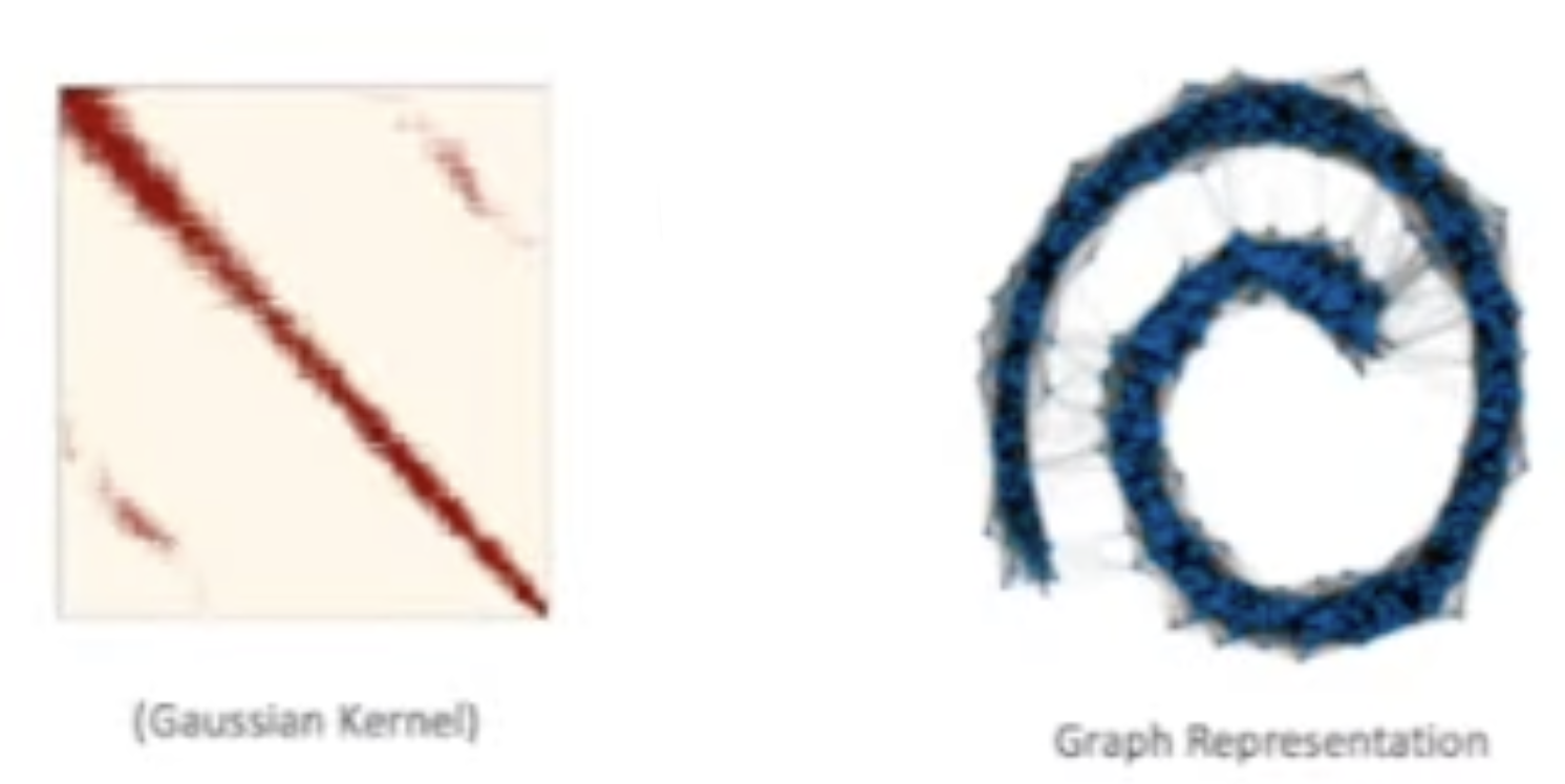

Affinity matrix

</div>

Transition Matrix

The affinity matrix is then row-normalized to create the stochastic transition matrix $P = D^{-1} A$, the affinity matrix pre-multiplied by the degree inverse matrix. This matrix defines the probability of a “random walk” jumping from one data point to another in a single step.

This transition matrix $P$ acts as a Diffusion Operator with several key properties:

1. Markov Chains: Diffusion operators define Markov Chains.
2. Assymetric: Because the operator is not necessarily symmetric, right eigenvectors ($Pu = \lambda u$) are generally unequal to left eigenvectors ($uP = \lambda u$).
3. Steady State: The left eigenvector corresponding to $\lambda = 1$ is the steady state vector. In Markov chain all the eigenvalues are less than or equal to 1.
4. Triviality: The right eigenvector corresponding to $\lambda = 1$ is trivial unless the graph is disconnected.
5. Powering: Powering a diffusion operator is mathematically equivalent to powering only its eigenvalues: \(P^t = U \Lambda^t U^{-1}\)

Heat Transfer

Why is $P$ called a diffusion operator? Because it diffuses heat! Since $P$ is a $n \times n$ matrix, it is a linear operator mapping a vector $f \in \mathbb{R}^n$ onto another vector in $\mathbb{R}^n$.

• Input: $f$ is a vector of length $n$, where each entry represents the “heat” at a specific data point. For example, if you put “1” at point $A$ and “0” everywhere else, you are starting with all the heat at point $A$.
• Operation: When you multiply the matrix $P$ by your vector ($P f$), the matrix acts as the diffusion operator. According to the transition probabilities in $P$, the heat at point $i$ is redistributed to its neighbors. Points that have high affinity (local similarity) receive more heat than points that are far away.
• Output: The output is a new $n$-vector, $f_{next} = Pf$. Each entry in this new vector contains the “updated” heat levels. If you repeat this $t$ times ($P^t f$), you are simulating the diffusion process over a specific time scale.

Eigendecomposition and Embedding

At this stage, diffusion map embedding also does eigendecomposition, but on a $n \times n$ matrix, not a $p \times p$ matrix. We compare the process with PCA.

1. Principal Component Analysis (PCA)

PCA operates on the feature space. We first compute the covariance matrix $\Sigma = \frac{1}{n-1}X^TX$, which is a $p \times p$ matrix. We then perform the eigendecomposition: \(\Sigma = U \Lambda U^T\) We retain the first $k$ components to form $U_k$. The low-dimensional embedding is then calculated via projection (inner product): \(X_{low} = XU_k\) By design, this imbedding preserves the covariance matrix.

2. Diffusion Map Embedding

In contrast, Diffusion Maps operate on the sample space. Here, we use a stochastic transition matrix $M$, which is $n \times n$ (where $n$ is the number of observations). Now each observation $X_i$ need not be $p$-dimensional Euclidean. It can be of any data type for which a kernel can be defined.

The eigenvector of $M$ is therefore an $n$-vector. For embedding, we do not project, but lookup and scale.

• For each observation $x_i$, we extract the $i$-th element from the first $k$ eigenvectors.
• After scaling by the eigenvalues $\lambda^t$ to account for the diffusion time, we arrive at the $k$-dimensional embedding: \(\Psi_t(x_i) = \left( \lambda_1^t \psi_1(i), \lambda_2^t \psi_2(i), \dots, \lambda_k^t \psi_k(i) \right)\)