Paper review: Building Representative Matched Samples With Multi-Valued Treatments in Large Observational Studies
A review of Magdelena Bennett et al. (2020) on using mixed-integer optimization to create representative matched samples for multi-valued treatments.
- Building representative matched samples with multi-valued treatments in large observational studiesJournal of Computational and Graphical Statistics, Apr 2020
Problem of interest
The 2010 Chile earthquake had a magnitude of 8.8 and caused more than 500 fatalities.

Introduction
Geographically, Chile lies along the Pacific Ring of Fire and experiences a major earthquake, on average, more than once every two years. Socially, Chile has the highest level of income inequality (as measured by the Gini index) among the 35 OECD countries, ranking above both Mexico and the United States.
In this context marked by extreme income inequality and recurring natural disasters, it is crucial to understand how such shocks affect college entrance examinations—the primary pathway for social mobility. Against this backdrop, the author—then a PhD student in education at Columbia University—sought to estimate the impact of this devastating earthquake on Chilean college entrance exam scores.
Causal effect
The causal effect cannot be identified simply by comparing the average test scores of students affected by the earthquake with those of students who were not. Suppose we observe that affected students score higher on average than unaffected students. This difference does not necessarily reflect the true impact of the earthquake. For instance, the areas hit by the earthquake may have been relatively wealthier and equipped with better educational resources, which could independently contribute to higher test scores.
The core principle of causal inference is that, to make a credible causal claim, the groups being compared must be equivalent in all relevant respects. Ideally, we would compare the same individual in two parallel worlds—one in which they experienced the earthquake and one in which they did not. Since such a comparison is impossible, we instead adjust for observable characteristics related to test performance and compare students who are as similar as possible along those dimensions.
Matching method
Matching provides one way to achieve this. It pairs units in the treatment group with comparable units in the control (or other treatment) group based on shared characteristics. In practice, units that cannot be adequately matched are often discarded, which reduces the sample size but improves comparability. After matching, we obtain pairs (or matched sets) of students who are similar in observed characteristics, making the comparison between them more credible.
Methodology
Data and method
The authors use census data from Chile. The dataset includes roughly 100,000 students. Treatment is defined as the level of earthquake exposure, measured in 10 levels. Each student is characterized by 14 categorical variables, including gender, ethnicity, parental education, and household income.
Multiple Treatments and the Template Dataset
When there are only two treatment levels, matching is relatively straightforward: one group can serve as the reference, and units from the other group are matched to it.
With multiple treatment levels, however, this approach is no longer sufficient. Instead, the authors construct a template population—a hypothetical set of students designed to represent the overall population characteristics of Chile. This template encodes the target distribution of covariates against which each treatment group will be matched.
MIP-Based Matching with Linear Size
The matching procedure is implemented using mixed-integer programming (MIP). Because the procedure is identical for each exposure level, we can focus on a single treatment level without loss of generality.
The key constraints are as follows:
- Each template unit must be matched to exactly one observed unit from the given treatment level.
- Each observed unit can be matched to at most one template unit (no reuse).
- For every covariate category, the number of matched observed units should mirror the number of template units in that category.
We can think of the data as arranged in a $P \times K$ grid, where rows represent covariates and columns represent categories. Each cell corresponds to a specific covariate-category combination. The template units are already distributed across these cells. The goal of matching is to “fill” the grid with treated units so that the distribution of matched units closely replicates that of the template.
This approach is known as cardinality matching, as it aims to balance the counts (cardinalities) within each cell. Formally, the optimization problem minimizes the total discrepancy in cell counts between the matched treated units and the template.
By minimizing this aggregate imbalance, the resulting matched sample of treated units becomes a representative reflection of the template population.
MIP of quadratic order of dataset size
Without loss of generality, we focus on a single treatment level, as the matching procedure remains identical across all levels.
Notations
The study involves units (e.g., students) defined by an outcome, a treatment status, and a set of covariates. We consider $P$ categorical covariates, $\mathcal{P} = {p_1, \ldots, p_P}$. Note that continuous variables, such as household income, are discretized into categories in this paper.
In the paper’s running example, the covariates include categorical variables such as gender, ethnicity, parental education levels, and household income. While each covariate in practice has a distinct number of levels, for ease of exposition we assume that each has exactly $K$ categories. Accordingly, each unit $i$ is represented by a covariate vector, for example, $\mathbf{x}_i \in [K]^P$.
The data is organized into two distinct sets:
- Treatment Dataset ($\mathcal{L}$): Units that received the specific treatment level under study. We denote this set as $\mathcal{L} = {\ell_1, \ldots, \ell_L}$. For example, a unit $\ell \in \mathcal{L}$ consists of an outcome $y_{\ell}$, a treatment $A_{\ell}$, and a covariate vector $\mathbf{x}_{\ell}$.
- Template Dataset ($\mathcal{T}$): A sample drawn from the population that represents the target covariate distribution. We denote this set as $\mathcal{T} = {t_1, \ldots, t_T}$. Since this dataset is generated for matching purposes, we only care about the covariate vector $\mathbf{x}_{t}$ for a given unit $t \in \mathcal{T}$.
Problem Coefficients
For each covariate $p \in {1, \dots, P}$ and category $k \in {1, \dots, K}$, we define:
- $N_{p,k}$: The number of units in the template dataset $\mathcal{T}$ that belong to category $k$ of covariate $p$. These represent our target counts for a representative sample.
Decision Variables
The optimization model uses two types of variables:
- $m_{t,\ell} \in {0, 1}$: A binary indicator that is $1$ if template unit $t \in \mathcal{T}$ is matched to treated unit $\ell \in \mathcal{L}$, and $0$ otherwise.
- $v_{p,k} \geq 0$: A continuous variable representing the “cell count margin”—the absolute difference between the number of matched treated units and the target count $N_{p,k}$. Because this margin is not restricted to integer values, the model is formulated as a mixed-integer linear programming (MILP) problem.
Constraints
The core logic of the model is captured in the following constraints:
-
Count Balance: This constraint connects the matching decisions ($m$) to the discrepancy margins ($v$): \(| \sum_{\ell \in \mathcal{L}_{p,k}} \left( \sum_{t \in \mathcal{T}} m_{t,\ell} \right) - N_{p,k} | \leq v_{p,k}\) where $\mathcal{L}_{p,k}$ is the subset of treated units possessing category $k$ of covariate $p$.
-
Matching Requirements: These ensure a valid one-to-one mapping without replacement:
- Each treated unit is matched at most once: $\sum_{t \in \mathcal{T}} m_{t,\ell} \leq 1, \quad \forall \ell \in \mathcal{L}$
- Each template unit is matched exactly once: $\sum_{\ell \in \mathcal{L}} m_{t,\ell} = 1, \quad \forall t \in \mathcal{T}$
Collecting everything together, the optimization problem is:
$$ \begin{aligned} \min_{\mathbf{v}, \mathbf{m}} \quad & \sum_{p=1}^{P} \sum_{k=1}^{K} v_{p,k} \\ \text{s.t.} \quad & \left| \sum_{\ell \in \mathcal{L}_{p,k}} \left( \sum_{t \in \mathcal{T}} m_{t,\ell} \right) - N_{p,k} \right| \leq v_{p,k}, \quad & \forall p \in \{1, \dots, P\}, \forall k \in \{1, \dots, K\} \\ & \sum_{t \in \mathcal{T}} m_{t,\ell} \leq 1, \quad & \forall \ell \in \mathcal{L} \\ & \sum_{\ell \in \mathcal{L}} m_{t,\ell} = 1, \quad & \forall t \in \mathcal{T} \\ & m_{t,\ell} \in \{0, 1\}, \quad & \forall t \in \mathcal{T}, \forall \ell \in \mathcal{L} \end{aligned} $$
Scalability: Variable and Constraint Complexity
While the MILP formulation is mathematically rigorous, it faces significant scalability hurdles. Specifically, the problem requires $T \times L + P \times K$ decision variables and a corresponding number of constraints. Since the matching variables grow quadratically with the number of units ($T \times L$), memory consumption in solvers like Gurobi can become a critical bottleneck for large-scale observational studies.
MIP of Linear Order Relative to Dataset Size
To improve scalability, the paper proposes a reformulation that reduces the number of decision variables. We define a new binary indicator $z_\ell = \sum_{t \in \mathcal{T}} m_{t,\ell}$ for each treated unit $\ell \in \mathcal{L}$.
The paper demonstrates that the constraint $m_{t,\ell} \in {0, 1}$ for all $t, \ell$ can be effectively replaced by a single binary constraint $z_\ell \in {0, 1}$ and a total count constraint $\sum_{\ell \in \mathcal{L}} z_\ell = T$. This argument leverages the fact that the matching requirements are equality constraints, allowing the problem to be solved without lose of generality in terms of matching. The resulting optimization problem is significantly more efficient:
$$ \begin{aligned} \min_{\mathbf{v}, \mathbf{z}} \quad & \sum_{p=1}^{P} \sum_{k=1}^{K} v_{p,k} \\ \text{s.t.} \quad & \left| \sum_{\ell \in \mathcal{L}_{p,k}} z_\ell - N_{p,k} \right| \leq v_{p,k}, \quad & \forall p, k \\ & \sum_{\ell \in \mathcal{L}} z_\ell = T \\ & z_\ell \in \{0, 1\}, \quad & \forall \ell \in \mathcal{L} \end{aligned} $$
Here, $z_\ell$ is a binary decision variable that takes the value 1 if treated unit $\ell$ matched by a template unit, and 0 otherwise.
Theoretical Guarantees of the Linear Formulation
A Mixed-Integer Program (MIP) is considered integral if its Linear Programming (LP) relaxation naturally yields an integer-optimal solution. The difference between the optimal objective value of the original integer problem and that of its LP relaxation is known as the integrality gap (or LP gap).
By shifting from a quadratic-size to a linear-size formulation, we do not sacrifice the tightness of the model. This is formalized in the following two propositions:
Proposition 4.1 (Equivalence of LP Gaps) The linear-size MIP and the quadratic-size MIP share the exact same LP gap. Consequently, the linear-size formulation is integral whenever the quadratic-size formulation is integral.
Proposition 4.2 (Integrality Guarantee for Two Covariates) In scenarios where there are at most two covariates, the linear-size MIP is strictly integral.
Results
Tables 1 and 2: Computational Speed
Tables 1 and 2 compare computational performance across different data sizes and levels of treatment granularity.
-
Formulation 1 (quadratic size): Produced an out-of-memory error with 32GB of RAM in Gurobi v7.5.1.
-
Formulation 2 (linear size): Successfully runs in R.
Table 1 varies the template size from 1,000 to 10,000 and the total sample size from 70,000 to 700,000. The linear formulation remained scalable across all settings, with average computation time increasing from approximately 0.2 minutes (70,000 observations) to 3.5 minutes (700,000 observations).
Table 2 fixes the template size at 1,000 and varies the total sample size from about 10,000 to 70,000, while also considering different numbers of exposure levels (3, 5, and 10). In all cases, the average computation time was under 0.3 minutes.
Together, these results demonstrate the substantial efficiency gains achieved by the linear-sized formulation.
Table 3: Imbalance Measure
Table 3 reports covariate imbalance under different numbers of treatment levels (3, 5, and 10).
In all settings, the procedure achieved exact matching, meaning the objective value was zero in every case. This indicates that the matched samples perfectly replicated the template distribution across all covariate categories.
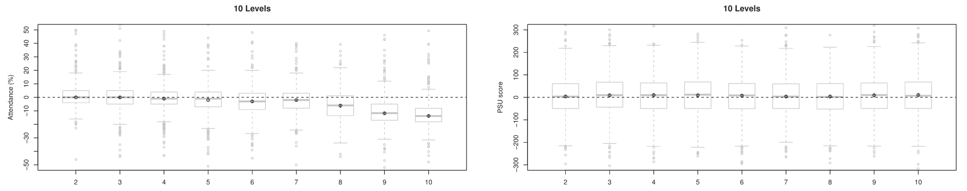
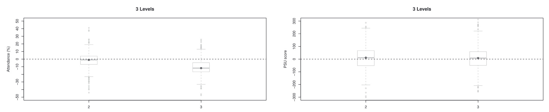
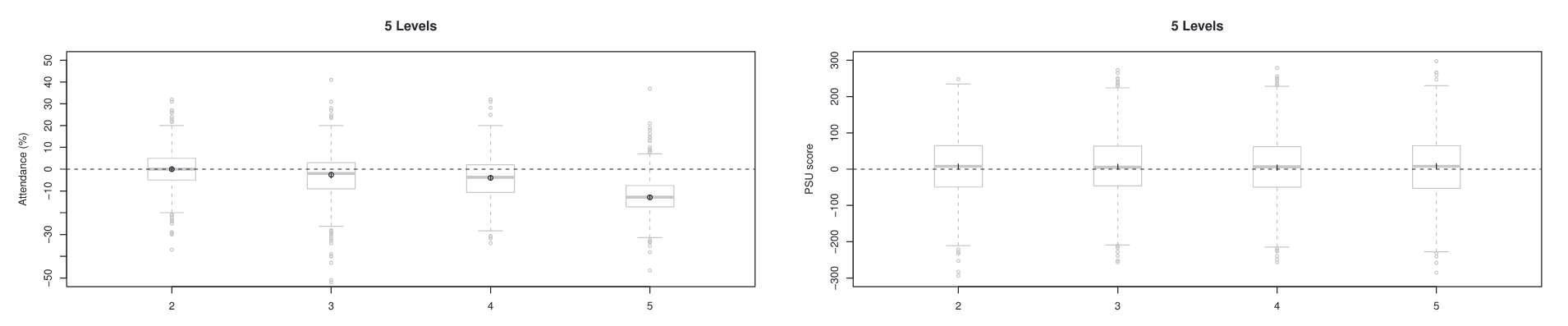
Figure 2: Visualization of Causal Effects
Figure 2 presents the estimated causal effects. The target matched sample size was approximately 1,000 students, and the procedure was repeated using different random seeds to assess stability.
Two outcomes were examined: attendance and test scores. Interestingly, the earthquake had a measurable effect on attendance but showed no significant effect on test scores.
three exposure levels
five exposure levels
ten exposure levels