The Illustrated Transformer

A visual explanation of the Transformer model, its components, and how it works.

Note: This post is a copy of Jay Alammar’s excellent The Illustrated Transformer, adapted for this blog.

In the previous post, we looked at Attention – a ubiquitous method in modern deep learning models. Attention is a concept that helped improve the performance of neural machine translation applications. In this post, we will look at The Transformer – a model that uses attention to boost the speed with which these models can be trained. The Transformer outperforms the Google Neural Machine Translation model in specific tasks. The biggest benefit, however, comes from how The Transformer lends itself to parallelization. It is in fact Google Cloud’s recommendation to use The Transformer as a reference model to use their Cloud TPU offering. So let’s try to break the model apart and look at how it functions.

The Transformer was proposed in the paper Attention is All You Need. A TensorFlow implementation of it is available as a part of the Tensor2Tensor package. Harvard’s NLP group created a guide annotating the paper with PyTorch implementation. In this post, we will attempt to oversimplify things a bit and introduce the concepts one by one to hopefully make it easier to understand to people without in-depth knowledge of the subject matter.

A High-Level Look

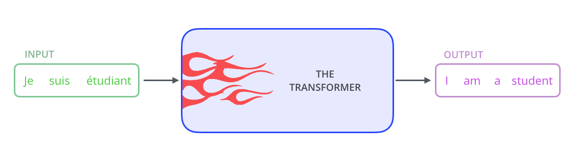
Let’s begin by looking at the model as a single black box. In a machine translation application, it would take a sentence in one language, and output its translation in another.

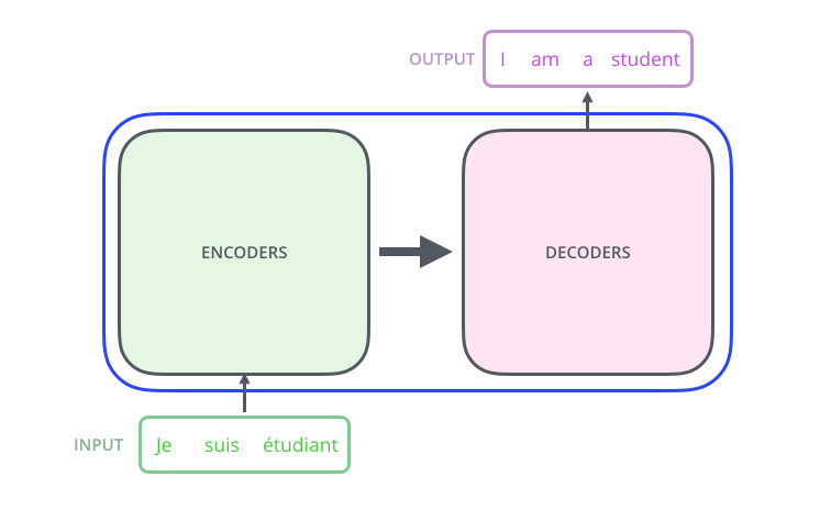
Popping open that Optimus Prime goodness, we see an encoding component, a decoding component, and connections between them.

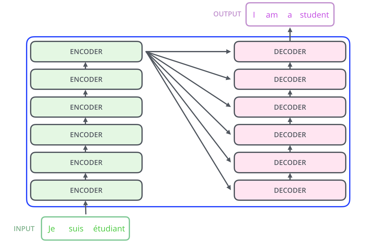
The encoding component is a stack of encoders. The paper stacks six of them on top of each other. Six is just an arbitrary number. Output of each encoder goes to *all decoders as their inputs. Output of the encoder is the contextual embedding. The decoding component is a stack of decoders of the same number.

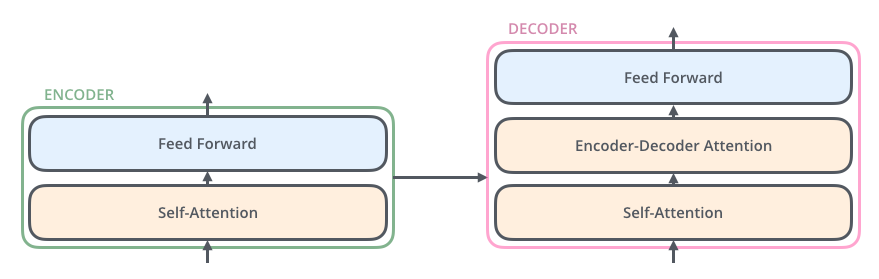
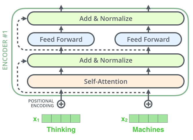
The encoders are all identical in structure (yet they do not share weights). Each one is broken down into two sub-layers:

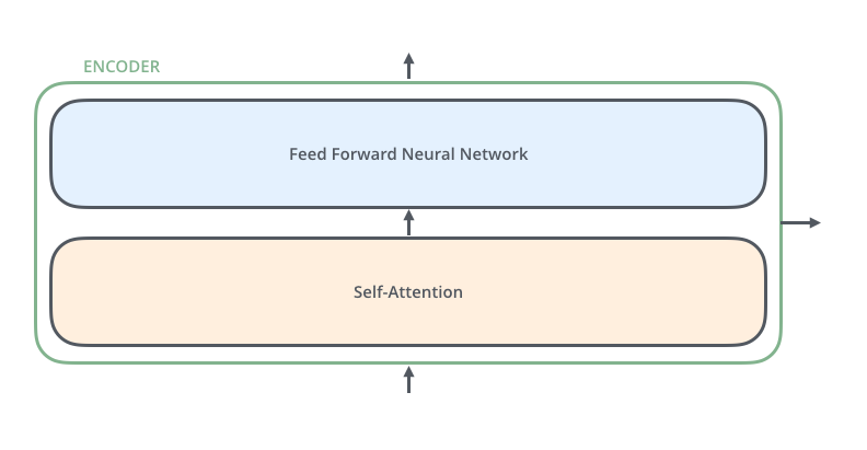
The encoder’s inputs first flow through a self-attention layer – a layer that helps the encoder look at other words in the input sentence as it encodes a specific word. We’ll look closer at self-attention later in the post.

The outputs of the self-attention layer are fed to a feed-forward neural network. The exact same feed-forward network is independently applied to each position.

The decoder has both those layers, but between them is an attention layer that helps the decoder focus on relevant parts of the input sentence (similar what attention does in seq2seq models).

Bringing The Tensors Into The Picture

Now that we’ve seen the major components of the model, let’s start to look at the various vectors/tensors and how they flow between these components to turn the input of a trained model into an output.

As is the case in NLP applications in general, we begin by turning each input word into a vector using an embedding algorithm.

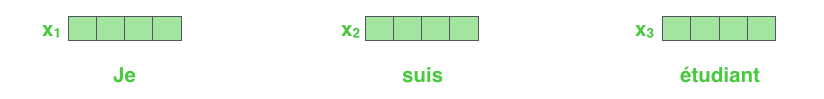
The embedding only happens in the bottom-most encoder. The abstraction that is common to all the encoders is that they receive a list of vectors each of the size 512 – In the bottom encoder that would be the word embeddings, but in other encoders, it would be the output of the encoder that’s directly below. The size of this list is hyperparameter we can set – basically it would be the length of the longest sentence in our training dataset.

Thus let’s focus on the non-bottom encoder. After embedding the words in our input sequence, each of them flows through each of the two layers of the encoder.

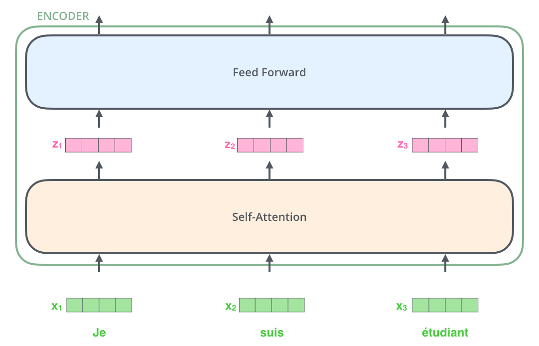
Here we begin to see one key property of the Transformer, which is that the word in each position flows through its own path in the encoder. There are dependencies between these paths in the self-attention layer. The feed-forward layer does not have those dependencies, however, and thus the various paths can be executed in parallel while flowing through the feed-forward layer.

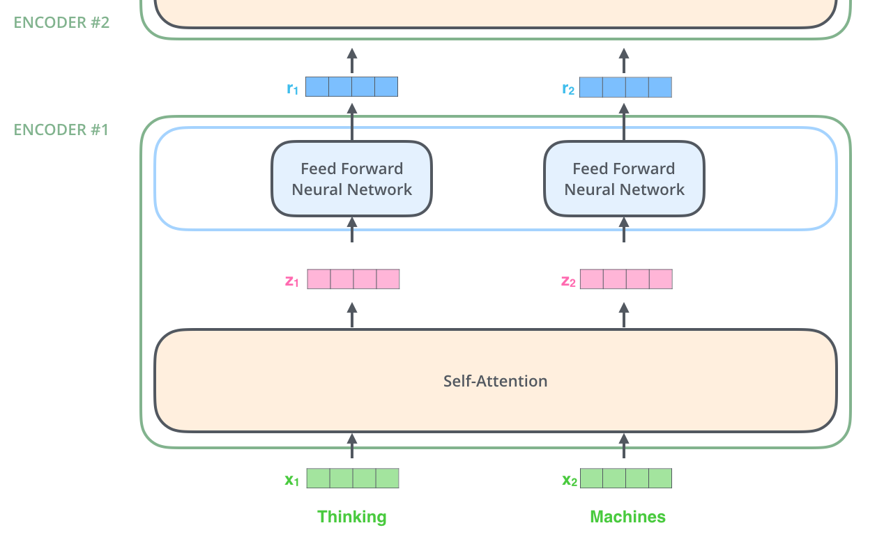
Now We’re Encoding!

As we’ve mentioned already, an encoder receives a list of vectors as input. It processes this list by passing these vectors into a ‘self-attention’ layer, then into a feed-forward neural network, then sends out the output upwards to the next encoder.

Self-Attention at a High Level

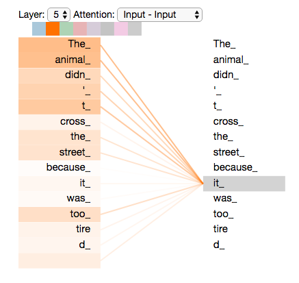
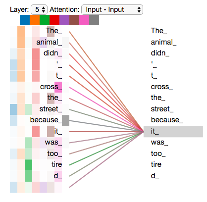
Say the following sentence is an input sentence we want to translate: ”The animal didn’t cross the street because it was too tired”

What does “it” in this sentence refer to? Is it referring to the street or to the animal? It’s a simple question to a human, but not as simple to an algorithm. When the model is processing the word “it”, self-attention allows it to associate “it” with “animal”. As the model processes each word (each position in the input sequence), self attention allows it to look at other positions in the input sequence for clues that can help lead to a better encoding for this word.

Self-Attention in Detail

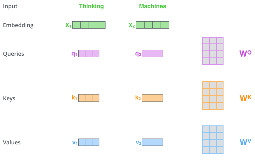
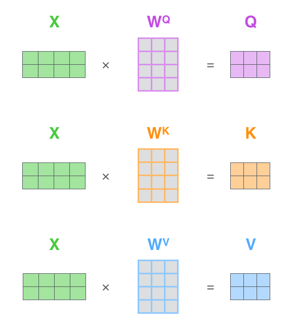
The first step in calculating self-attention is to create three vectors from each of the encoder’s input vectors (in this case, the embedding of each word). So for each word, we create a Query vector, a Key vector, and a Value vector. These vectors are created by multiplying the embedding by three matrices that we trained during the training process.

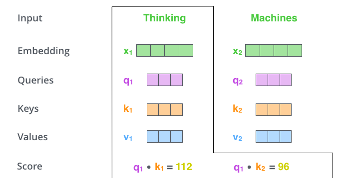
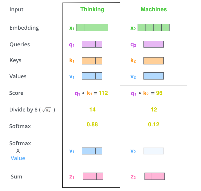
The second step in calculating self-attention is to calculate a score. Say we’re calculating the self-attention for the first word in this example, “Thinking”. We need to score each word of the input sentence against this word. The score determines how much focus to place on other parts of the input sentence as we encode a word at a certain position.

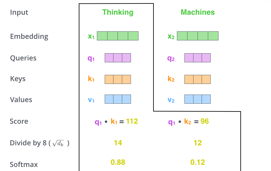
The third and fourth steps are to divide the scores by 8 (the square root of the dimension of the key vectors used in the paper – 64), then pass the result through a softmax operation. Softmax normalizes the scores so they’re all positive and add up to 1.

The fifth step is to multiply each value vector by the softmax score. The intuition here is to keep intact the values of the word(s) we want to focus on, and drown-out irrelevant words.

The sixth step is to sum up the weighted value vectors. This produces the output of the self-attention layer at this position (for the first word).

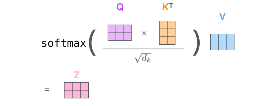
Matrix Calculation of Self-Attention

In the actual implementation, the calculation is done in matrix form for faster processing.

The Beast With Many Heads

The paper further refined the self-attention layer by adding a mechanism called “multi-headed” attention. This improves the performance of the attention layer by:

1. Expanding the model’s ability to focus on different positions.
2. Giving the attention layer multiple “representation subspaces”.

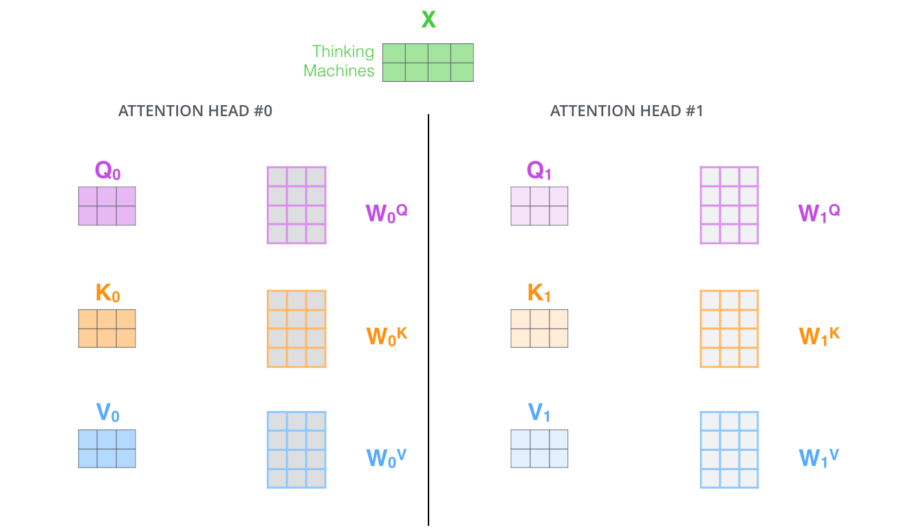
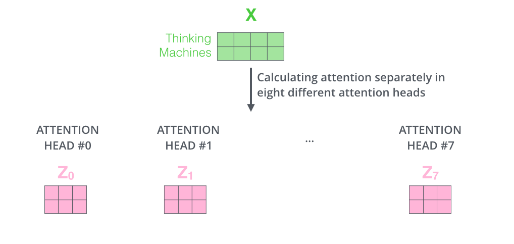
If we do the same self-attention calculation we outlined above, just eight different times with different weight matrices, we end up with eight different Z matrices.

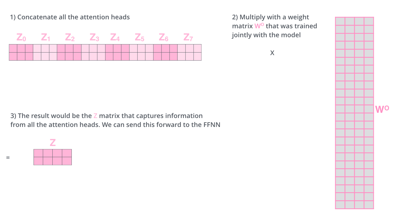
We concat the matrices then multiply them by an additional weights matrix WO to condense them into a single matrix.

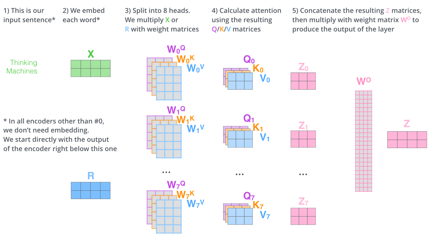
Here is a visual recap of the multi-headed self-attention:

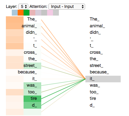
Now let’s revisit our example to see where the different attention heads are focusing as we encode the word “it”:

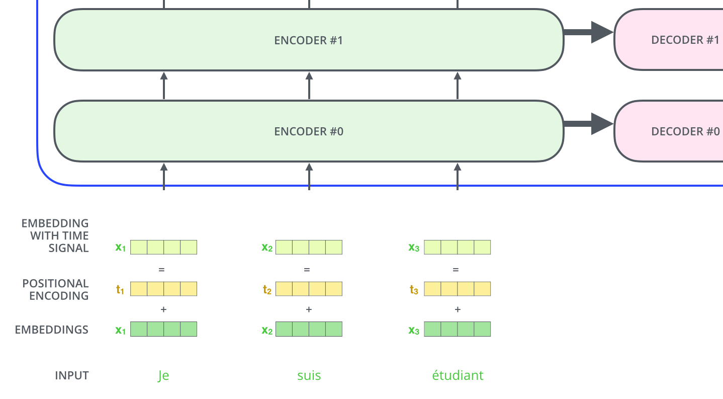
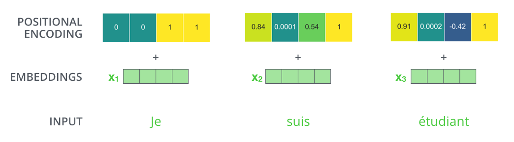
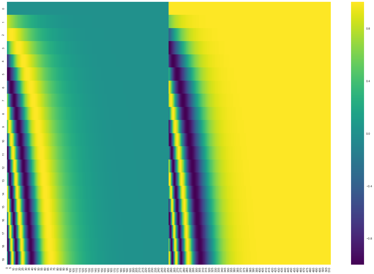
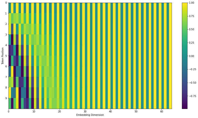
Representing The Order of The Sequence Using Positional Encoding

To account for the order of words, the transformer adds a vector to each input embedding.

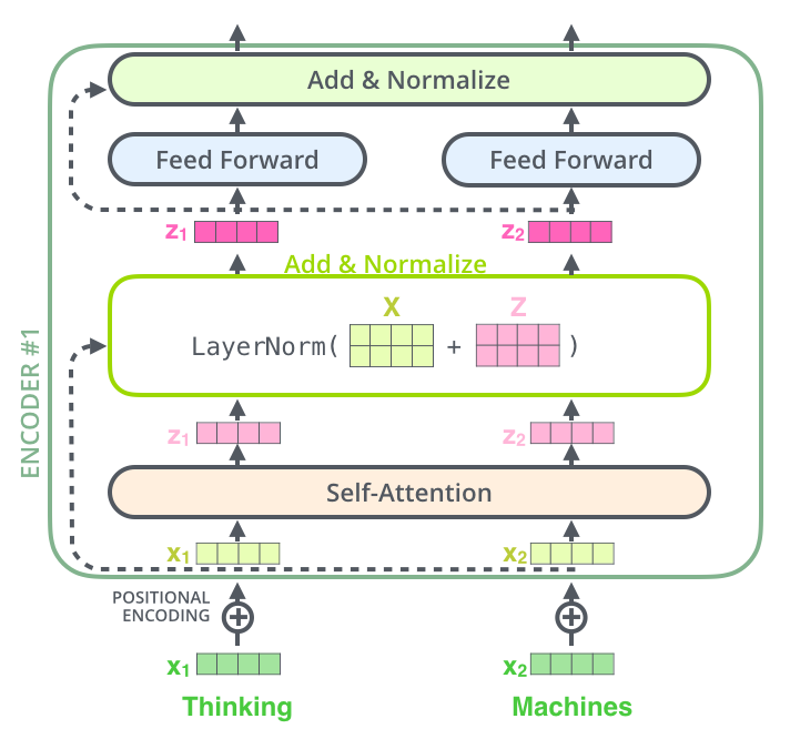
The Residuals

Each sub-layer in each encoder has a residual connection around it, followed by a layer-normalization step.

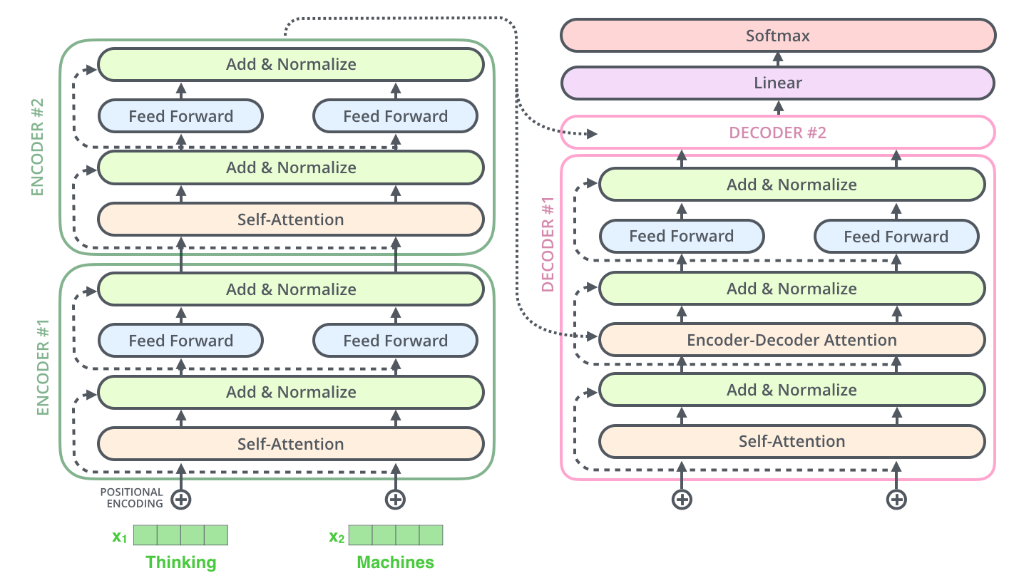
The Decoder Side

The encoder start by processing the input sequence. The output of the top encoder is then transformed into a set of attention vectors K and V. These are to be used by each decoder in its “encoder-decoder attention” layer:

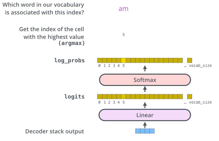
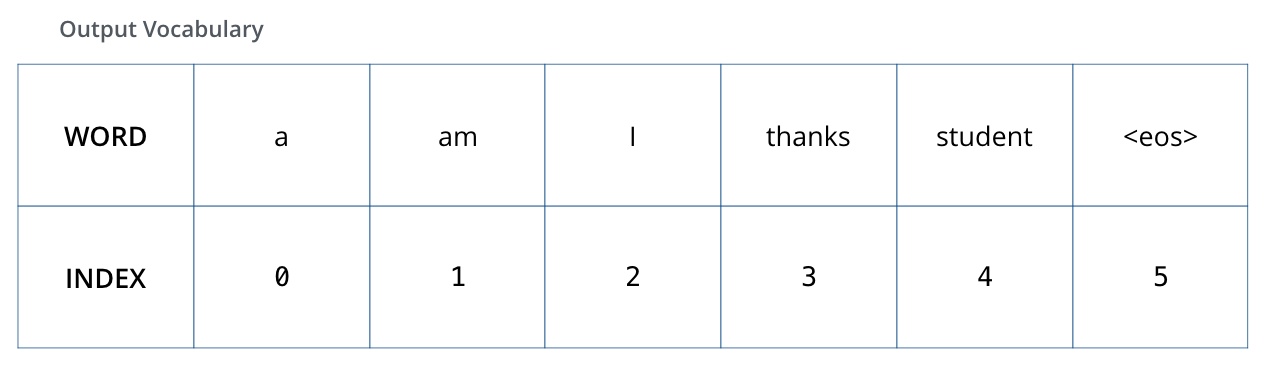
The Final Linear and Softmax Layer

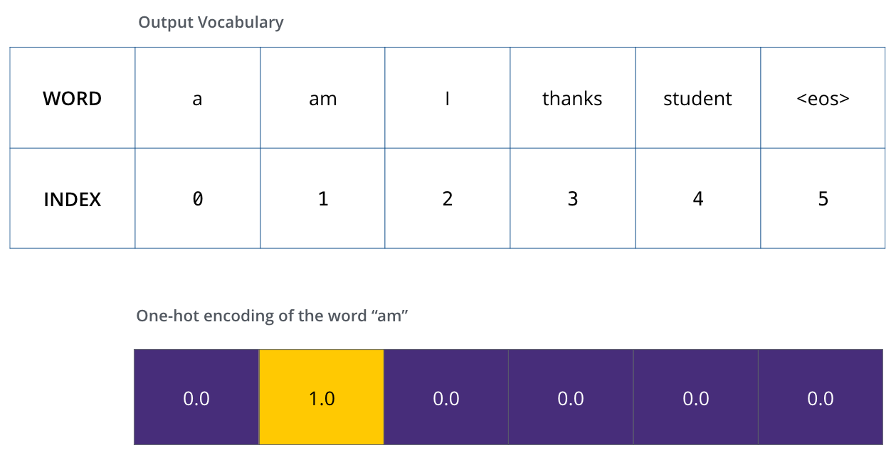
The decoder stack outputs a vector of floats. The final Linear layer followed by a Softmax Layer turns that into a word.

Recap Of Training

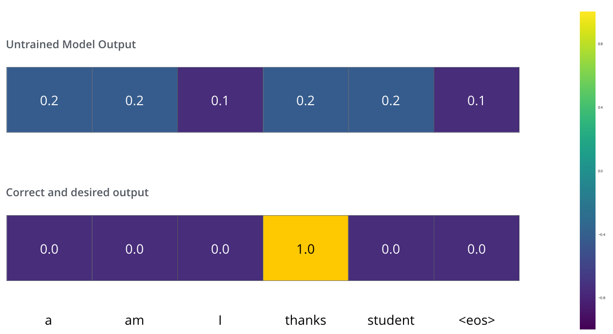
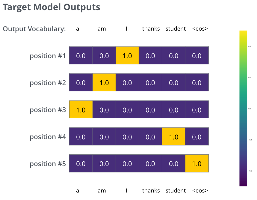
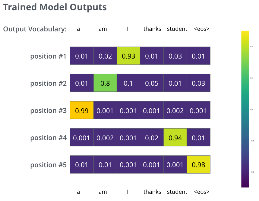
During training, we compare the model’s output with the actual correct output.

The Loss Function

We aim to minimize the cross-entropy loss between the predicted probability distribution and the ground truth.

Problem Setup

In self-attention, (Q), (K), and (V) all derive from the same input sequence of length (n). Given the following matrices with sequence length (n = 2) and dimension (d_k = 2):

Query

\[Q = \begin{bmatrix} 1 & 2 \\ 0 & 1 \end{bmatrix}\]

Key

\[K = \begin{bmatrix} 1 & 1 \\ 0 & 1 \end{bmatrix}\]

Value

\[V = \begin{bmatrix} 5 & 0 \\ 0 & 5 \end{bmatrix}\]

Each row represents a token in the sequence. (Q[i]) is the query for token (i), (K[j]) is the key for token (j), and (V[j]) is the value for token (j).