1. Data Collection and Preprocessing

The study combines two distinct datasets to create a predictive model:

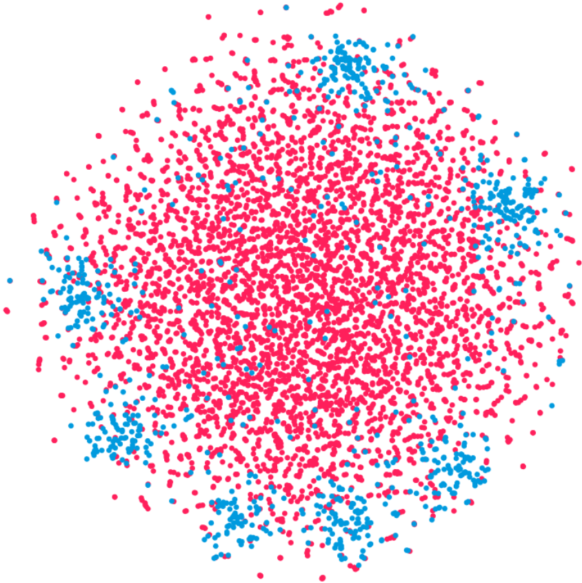
• ROKA Dataset: Obtained from the Republic of Korea Army, this dataset records 984 artillery training sessions over five years. It provides the binary response variable: wildfire occurrence ($1$) or non-occurrence ($-1$). The data is highly imbalanced, with a ratio of approximately 1:24 (40 fires vs. 944 non-fires).
• SKMA Dataset: Sourced from the South Korea Meteorological Administration, this provides meteorological predictor variables including temperature, precipitation, wind speed, and relative humidity.
• Data Merging and Normalization: The datasets were linked via temporal information. To account for the distance between weather stations and training sites, the study used Barnes interpolation to create a gridified weather map. Additionally, a Digital Elevation Model (DEM) was used to normalize temperature data based on the altitude differences between observation stations and training sites. All predictor variables were normalized to have a zero mean and a standard deviation of one.

2. Proposed Algorithm: GC-WSVM

The authors proposed a method called Gaussian mixture clustering weighted SVM (GC-WSVM), which operates in two steps to handle the skewed class distribution:

• Step 1: GMM-Based Oversampling:
  • The study utilized a Gaussian Mixture Model (GMM) to estimate the probability distribution of the minority class (wildfire occurrences).
  • Synthetic samples were generated from this learned distribution to balance the dataset.
  • GMM was chosen over the traditional SMOTE algorithm because the minority class samples exhibited a clustered structure, and SMOTE’s linear interpolation could incorrectly generate samples in the empty space between subgroups.
• Step 2: Weighted Support Vector Machine (WSVM):
  • A weighted Gaussian kernel SVM was applied to the balanced dataset.
  • The algorithm assigned different misclassification costs (weights) to the classes.
  • To prioritize the detection of the minority class, the weights were set proportional to the inverse of the number of samples; specifically, the cost for misclassifying a wildfire ($1/n_{min}^*$) was set higher than that for non-occurrence ($1/n_{maj}$).

3. Experimental Design and Validation

• Comparison: The performance of GC-WSVM was compared against Linear SVM and standard Gaussian Kernel SVM.
• Validation Method: Due to the scarcity of minority samples, the study employed fivefold cross-validation rather than a simple train-test split.
• Hyperparameter Tuning: A grid search was conducted to tune hyperparameters, including the cost parameter $C$, the Gaussian kernel bandwidth $\gamma$, and the desired imbalance ratio $R$.
• Metrics: The model performance was evaluated using Sensitivity, Specificity, and the $G-mean$ (the geometric mean of sensitivity and specificity), as the latter provides a balanced view of performance on both majority and minority classes. rather than a simple train-test split[cite: 424, 425].
• [cite_start]Hyperparameter Tuning: A grid search was conducted to tune hyperparameters, including the cost parameter $C$, the Gaussian kernel bandwidth $\gamma$, and the desired imbalance ratio $R$[cite: 430, 431].
• [cite_start]Metrics: The model performance was evaluated using Sensitivity, Specificity, and the $G-mean$ (the geometric mean of sensitivity and specificity), as the latter provides a balanced view of performance on both majority and minority classes[cite: 185, 186].

Challenges and Methods

1. XY-axis Interpolation: Barnes Interpolation

Challenge: A significant spatial discrepancy exists between KMA weather observatories and artillery training sites. To accurately estimate meteorological conditions at specific training locations, spatial interpolation is required.

Method Intuition: The study employs Barnes Interpolation, which functions essentially as a two-step Nadaraya-Watson (NW) estimation process. It addresses the high bias (over-smoothing) typical of a single kernel smoother by introducing a second estimator to correct local errors.

Step 1: The Initial Estimate (Base Learner)

The first pass utilizes a standard Nadaraya-Watson estimator with a Gaussian kernel.

• Goal: Capture the field’s global trends (e.g., general pressure systems).
• Mechanism: Estimates the value at any grid point, $g_0(x)$, via a weighted average of surrounding observed data points, $f_k$.
• The Kernel: Weights are determined by a Gaussian kernel with bandwidth $\kappa$.
  • $g_0(x) \approx \text{Weighted Average of Neighbors}$

Step 2: The Correction (Residual Learner)

The second pass applies a Nadaraya-Watson estimator to the residuals.

• Goal: Recover local, high-frequency details (e.g., small storm pockets) smoothed over by the first pass.
• Mechanism:
  1. Calculate the residual at every original data point: \(Error = \text{Observed Value} - \text{First Pass Estimate}\)
  2. Apply a second NW estimator to these error values.
• The Kernel Adjustment: This pass uses a narrower bandwidth (scaled by $\gamma$, where $0.2 < \gamma < 1.0$) to capture the sharp, local variations missed by the broader first kernel.

Final Result

The final interpolated map combines the global trend with the local correction:

2. Z-axis Interpolation for Temperature

Challenge: In addition to horizontal distance, the altitude of weather stations often differs significantly from that of the training sites. Since temperature changes with elevation, using raw station data without adjustment would introduce significant error.

Method Intuition:

• Step 1: Acquiring Elevation Data Since the Army dataset lacks altitude information, the study utilizes an open-source digital topographic database of Earth from the Shuttle Radar Topography Mission (SRTM). This dataset provides high-resolution elevation data (30 meters) (Source: OpenTopography)

• Step 2: Lapse Rate Adjustment The temperature recorded at the observation station is adjusted using a standard lapse rate of $0.65^\circ\text{C} / 100\text{m}$.

3. Minority class oversampling

SMOTE (Synthetic Minority Oversampling Technique)

For each actual minority class sample (let’s call it Point A), given a tuning paramete $k$:

1. Find Neighbors: It looks around Point A and identifies its $k$ nearest minority class neighbors.
2. Pick a Partner: It randomly chooses one of those neighbors (let’s call it Point B).
3. Draw a Line: Imagine drawing a straight line connecting Point A and Point B.
4. Create a New Point: The algorithm picks a random spot somewhere along that line and places a new, synthetic point there.

Why the Authors Rejected It

Visual inspection revealed that the wildfire data was clustered into subgroups. This creates a risk for SMOTE: if Point A belongs to one subgroup and one of its $k$ “nearest neighbors” (Point B) belongs to a separate subgroup nearby, SMOTE will draw a line connecting them through the empty space between clusters. Any synthetic point generated along this line would likely be unrealistic, representing a data point that does not statistically resemble a real wildfire event.

Gaussian Mixture Model (GMM)

GMM is a probabilistic model that assumes all data points are generated from a mixture of a finite number of Gaussian (normal) distributions with unknown parameters.

• In this paper: The authors observed that the minority class (wildfire occurrences) formed several distinct clusters rather than a single group.
• Application: Instead of assuming a single distribution, they used GMM to estimate the probability distribution of these minority samples. They then generated synthetic data from this learned distribution to oversample the minority class and balance the dataset.

5. SVM (Support Vector Machine)

Support Vector Machine (SVM) is a supervised classifier that identifies the optimal hyperplane ($w \cdot x + b$) by optimizing the sum of two conflicting objectives: hinge loss and squared $\ell_2$ regularization. The hinge loss penalizes the model for misclassifying points; it earns its name because correctly classifying points (outside the margin) incurs zero loss, whereas misclassification incurs a linear loss proportional to the distance from the boundary. Meanwhile, the squared regularization minimizes the norm of the weights ($|w|^2$), which is mathematically equivalent to maximizing the margin—the geometric distance between the decision boundary and the nearest data points. Notably, since the mathematical formulation relies entirely on inner products between data points, the linear decision boundary can be extended to capture nonlinear relationships by replacing these inner products with a kernel—a bivariate, nonlinear function that maps two points to a measure of their similarity in a higher-dimensional space.

7. Weighted SVM

To prevent the model from overlooking rare wildfire incidents, the weighted SVM modifies the learning algorithm by adjusting the hyperplane towards the minority class, which helps classify more samples as part of that group. It does this by adjusting the slope of the hinge loss function separately for the positive and negative classes. Specifically, the weights are set proportional to the inverse of the number of original samples, effectively making the model “pay more” for misclassifying a wildfire.

Furthermore, our follow-up research proposes utilizing three distinct hinge loss functions corresponding to the original majority class, the original minority class, and the synthetic minority class. The slopes of these losses are scaled according to the ratio of the total majority class to the total minority class, and the ratio of synthetic minority samples to original minority samples.

We demonstrate that as the original sample size approaches infinity—assuming the Gaussian Mixture Model sufficiently approximates the minority class distribution and the oversampling and weighting policies remain fixed—this SVM converges to the Bayes optimal classifier. This result establishes statistical consistency rather than optimality; it satisfies the minimum requirement of a learning algorithm: given infinite data, the algorithm recovers the best theoretically possible decision boundary (the Bayes classifier). The proof follows a two-step logic:

1. Reduction to 1D Optimization: Utilizing the properties of Reproducing Kernel Hilbert Spaces (RKHS), the optimization over the population expectation is reduced to a one-dimensional optimization problem on the real line. This reduction generalizes the findings of Lin et al. (2002) to our specific framework incorporating three hinge losses.
2. ERM Convergence: Treating the SVM as an Empirical Risk Minimization (ERM) problem, we demonstrate that the solution to the ERM converges to the solution of the population optimization as approaches infinity.

Details of the Army dataset

The dataset tracks several key variables for each incident:

• Date: This captures the specific date and time of the event. The provided examples—spanning October, November, April, and March—align with the study’s finding that the vast majority of military wildfires (39 out of 40) occur during the dry seasons of February–April and October–November[cite: 196, 197, 237].
• Location: The administrative district where the training occurred is recorded, such as Goseong-gun or Paju-si.
• Shooting Type: This details the specific munition or weapon system that triggered the fire. Examples include:
  • Red parachute flare and Star shell (illumination rounds).
  • 60 mm trench mortar (artillery).
  • Panzerfaust3 (anti-tank warhead).
• Damaged Area: This measures the extent of the forest affected by the fire, with values in the provided examples ranging from 2,500 to 150,000.

Variable Exclusion and Future Work

It is important to note that while Location, Shooting Type, and Damaged Area appear in the raw data, the authors excluded them from the final predictive model. Location and Shooting Type were removed to focus the model strictly on meteorological conditions, while Damaged Area was ignored because the model functions as a binary classifier (predicting occurrence vs. non-occurrence) rather than a regression model predicting severity. However, the authors suggest that incorporating these variables could enhance predictive power and remains a potential avenue for future research.

Sample data

| No. | Date | Location | Cause (Shooting Type) | Damage Size | Fire Occurred | | :— | :— | :— | :— | :— | :— | | 1 | Oct 31, 2019 | Goseong-gun | Red parachute flare | 2,500 | 1 | | 2 | Nov 8, 2019 | Goseong-gun | Star shell | 3,000 | 1 | | 3 | Apr 13, 2017 | Paju-si | 60 mm trench mortar | 150,000 | 1 | | 4 | Mar 22, 2018 | Paju-si | Panzerfaust3 | 3,300 | 1 |